Use Cases of Serverless Pool

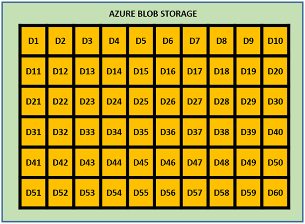
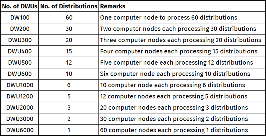
To achieve high query performance data must be distributed which help in running queries in parallel. When we store data in Synapse (dedicated SQL Pool) it's distributed across 60 fixed distributions (distributed location is called a distribution). Each of those distributions functions as an independent storage and processing unit that runs queries on its portion of the data.

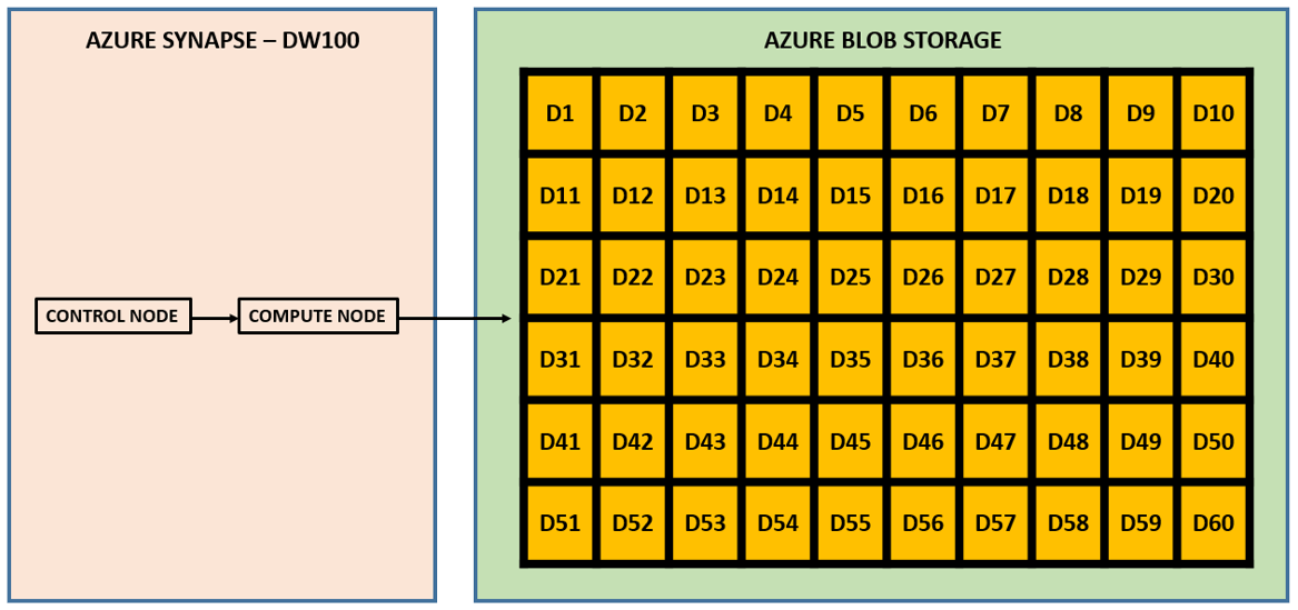
Number of distributions assigned to compute nodes gets changed every time when there is a change in number of compute nodes. For example, in the figure below, the size of the Synapse database is DW100 and hence there is only one compute node processing data for all those 60 distributions.

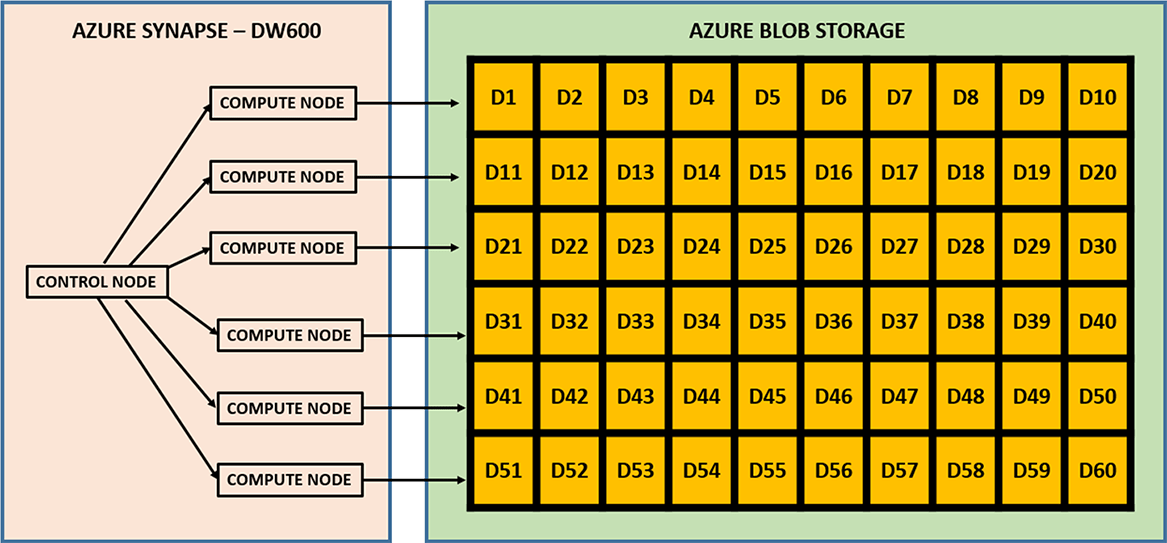
The number of compute nodes must divide 60 with zero remainder so that each compute node has an equal number of distributions to process.

  Data from each table is divided across 60 underlying databases, called distributions
  Table structure is identical in each distribution
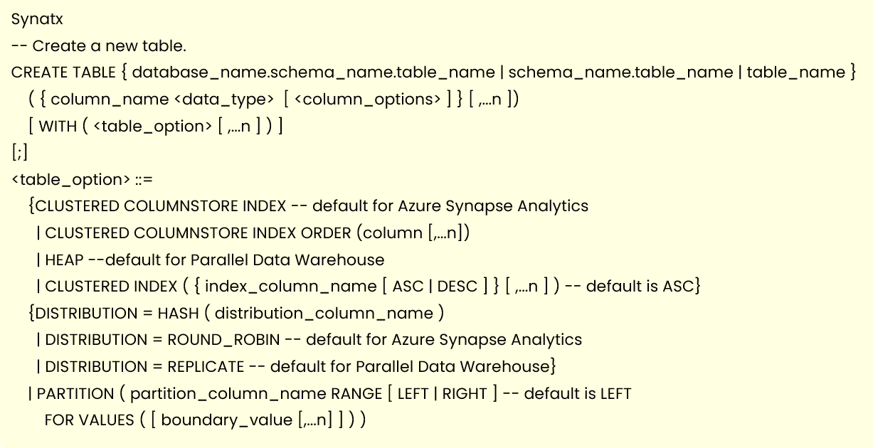
  We can specify distribution method during table creation: HASH, ROUND_ROBIN or Replicate
  Rows are allocated to distribution during data load based distribution method selected in CREATE TABLE statement

Serverless SQL Pool

  This is an auto-scale compute environment that uses T-SQL to query the data lake directly without the need to any data replication or staging the data. In this case data lake is used as the storage and Serverless SQL is being used as the compute
  It is used as query as a service (QaaS) over data lake storage
  Since it is Serverless, hence there's no infrastructure to setup or clusters to maintain. A default endpoint for this service is provided within every Azure Synapse workspace, so we can start querying data as soon as the synapse workspace is created
  Here we don’t have to provision a server, it auto-scales and we consume the service on a pay-per-query cost model
  Distributed Querying Processing (DQP) engine being used here that assigns tasks to compute nodes to finish the query execution
  Number of compute nodes decided based on the number of tasks determined by DQP engine. This is what allows Serverless SQL Pool to scale automatically any query requirement.
  Computation cost is based on per TB of data processed by the queries that we execute. Currently cost to process 1 TB of data is US 4.85$
  With Serverless SQL Pool we can query data stored in ADLS Gen2, Azure Blob Storage, Cosmos DB

Use Cases of Serverless Pool

  Explore and discover data in Azure Storage quickly and on-demand
  Create a Logical data warehouse by creating transformation views in a metadata store for up to data, directly querying from your raw ADLS Gen2 (Data Lake) storage layer
  Provide a relational abstraction on top of raw or disparate data without relocating and transforming data, allowing always up-to-date view of your data       a)  Data Transformation - Simple, scalable, and performant way to transform data in the lake using T-SQL, so it can be fed to BI and other tools, or loaded into a relational data store (Synapse SQL databases, Azure SQL Database, etc.).       b)  Build data visualization layers in Power BI, directly querying against Spark Tables.

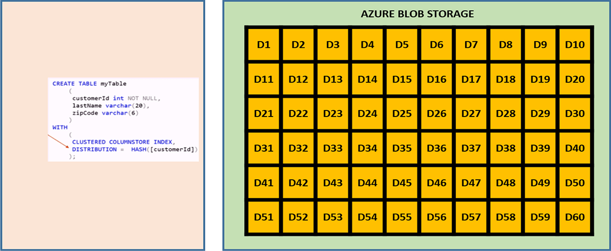
Hashing is a function where we input a number and it produces an output called the Hash Value. when we are inserting a row into a table using the table definition mentioned above, the value of the column "Customer ID" is going to get passed into a Hash function. In case it's deterministic each time you pass the same input value you will be getting the same Hash Value as an output. And if it's non-deterministic you pass in the same value and you get a different value. In Synapse it's always the same value generated. So it’s a deterministic Hash function. A hash distributed table can deliver the highest query performance for joins and aggregations on large tables.

The distribution column is what determines how the data is divided across your distributed databases. The hash function uses the distribution column to assign rows to distributions. The hashing algorithm and resulting distribution is deterministic. That is the same value with the same data type will always has to the same distribution.

Therefore, the column that is selected for the hash distribution should be chosen carefully. If a column is chosen on 10 million row table for the hash distribution. For example, there is a State column and 85% of the records in the State column has a value Maharashtra, then there would be an uneven spread of the data across the distributions. So we must select a column that has relative even distribution of data and a column that wouldn’t be updated.

Round-Robin Distribution

During table creation if we don’t specify any distribution type then be default “Round-Robin” distribution is going to be selected. This distribution method is fairly simple to setup but since we are not concerned about the location of the data across the distributions thus data movement during query execution become expensive and can affect the overall performance.

As a result, the system sometimes needs to invoke a data movement operation to better organize your data before it can resolve a query. This extra step can slow down your queries. For example, joining a round-robin table usually requires reshuffling the rows, which is a performance hit.

Consider using the round-robin distribution for your table in the following scenarios:

  When getting started as a simple starting point since it is the default
  If there is no joining key involved
  If there is no good candidate column for hash distributing the table
  If the table does not share a common join key with other tables
  If the join is less significant than other joins in the query
  When the table is a temporary staging table

Replicated Table Distribution

To avoid any data movement, we use replicated tables. Optimized query in an MPP executes on single distribution databases without any interaction with other distributions. But to satisfy join criteria in a query sometimes data movement is required between distributions. Replicated tables are tools that can be used to avoid data movement for small tables. It has a full copy which is accessible by each compute node. Replicating table removes the need to move the data among compute nodes before join/aggregation. They are good for small tables like dimensions in a star schema. A dimension table is is something that stores descriptive data that typically changes slowly, so things like customer name, address, or product key.

There are three storage modes available in Power BI to connect with Synapse
Import Mode – In this case table data is stored in-memory like a snapshot and data can be refreshed periodically (based on the incremental refresh option). This in-memory columnar storage is called VertiPaq.
DirectQuery Mode – Here we are extracting data directly from the source and not storing anything. Data resides in its original source before, during and after query execution
Dual or Composite Mode – It’s a combination of Import and DirectQuery mode. Data from the table is being loaded into memory, but at the query time it can be also retrieved directly from the source

With Synapse Link Services option we can take advantages of including whole set of different features and services existing external to Synapse like Azure Datalake, Amazon Redshift, CosmosDB etc.

Inside Manage Linked Services option we can even linked our Power BI Workspace which allows us to build Power BI reports immediately straight from Synapse Analytics Studio.

In Azure we have following services used widely –

  Data Ingestion - Azure Data Factory
  Data Storage - Azure DataLake Storage Gen2
  Data Transformation - Mapping data flows in ADF
  Data Model - Azure Synapse Analytics
  Data Visualization - Power BI is used to visualize the data

Below diagram shows how it works:

  Use Power BI Import Data option for all master data stored in Synapse
  In order to build Aggregation/Summary data we can select any one of the two options

Option #1 - Build multiple aggregation tables as Import Data option in Power BI itself
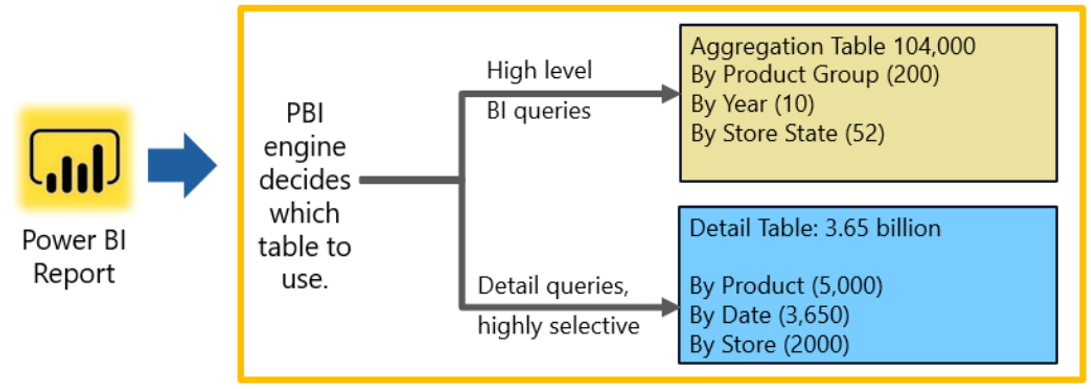
  To improve user experience while dealing with large datasets, aggregations are one of the modeling optimization technique being used. Combined with Power BI composite models, these modeling optimization techniques make it possible to analyze big datasets efficiently by allowing high level analytical queries to be answered from memory as part of the aggregation tables while sending more detailed queries back to the source database. In this case aggregation tables will be part of import data and for detailed queries use DirectQuery and let PBI engine decides which table to use based on the need.

In this design, the Aggregation table needs to be maintained as part of the overall database maintenance. When the main table is updated, the aggregation table needs to update as well (incremental refresh). In Power BI, aggregations start as a table just like any other table in a model. It can be based on a view or table in the source database, or created in Power BI with Power Query.

Two choices are there to implement -

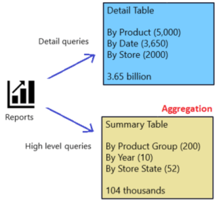
1) Detail and Aggregation tables both in DirectQuery mode
2) Detail table in DirectQuery mode and Aggregation table in Import Mode

Note - Build the aggregation tables at the database level and then import it to in-memory in PBI

Taking the benefit of Composite model where we're creating an aggregated table in Synapse and setting it up in Import mode considered to be most desirable scenario. Using this concept, your aggregated table will be stored in Power BI cache memory, optimally compressed, while your huge table with all the details will continue to reside in the Synapse Dedicated SQL pool

Option #2 - Build materialized view in Synapse and use it in Power BI either as DirectQuery or Import Data option

Materialized View works by saving the result of the query when it is created, rebuilt, or the underlying data is changed. Similar to the tables on the SQL Pool, the materialized views can be customized by their distribution, partitioning, and indexing. Unlike other Cloud Data Warehouses like Amazon Redshift, the materialized views on Synapse don't need to be refreshed manually with the new data coming in, this is done automatically by Synapse as the underlying data changes.

Benefit of using Materialized View in Power BI by using DirectQuery option.

In case of materialized views we will essentially aggregate the data but not import in Power BI, as we will target this view using DirectQuery mode. A materialized view is like a virtual table, but unlike a “standard” view, that computes data each time you use it, a materialized view instead pre-computes, stores and maintains its data in a Dedicated SQL pool like a regular table. So, we are getting a faster performance for our most frequent workloads, but as a trade-off, we’re paying the price for the additional storage in terms of materialized view.

Serverless SQL Pool is a query processing engine for datalake. Let say we have our data in data lake storage and assume that we’re going to store this data in parquet format. We will be querying the parquet files available in data lake storage from our Power BI reports.

Serverless Pool allows us to query multiple files from Azure DataLake using SQL like syntax.

If we execute this query, we can run the SQL query over the entire folder. Now that we've established that we can query the data, we need to create a SQL Serverless view which we will then be able to query from Power BI. First, we must create a SQL script for creating a new database within our Synapse account:

When we run this script we would be able to see the database. Once we have our database, we then run our second script which creates the view

We now have a view within our database which we will be able to query from within Power BI.

So we have three components here:

1) Azure Data Lake - for storing the data in parquet format
2) Azure Synapse - for creating SQL Serverless views over data stored in the data lake
3) Power BI - for querying the SQL Serverless views and creating visualizations over the data
(Note – Using SQL Serverless we can create logical data warehouse and connect with Power BI)